Rainy/Snowy Day Max: Spirographics
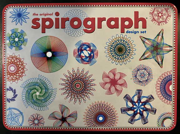
I'm sure a lot of you are going to look at this picture and be transported to childhood (either your own, or one of your own children or younger friends): The Spirograph. This deceptively simple collection of geared rings and wheels and pens were the source of hours of drawing fun; You pinned down the big ring, grabbed a little gear full of holes, put your pen in the hole of your choice, and your pen magically drew these amazing curves and shapes inside or outside of the toothed ring as you moved the little wheel on its circular path... that is, unless your hand slipped and the wheel came loose, in which case you started again and learned a little coordination as well as creating cool designs!
For this seasonally-appropriate edition of Rainy Day Max, we're going to revisit those exciting days of drawing by implementing a version of the Spirograph with Jitter using Javascript — we'll walk you how to conceptualize the mathematics of the hypotrochoids and epitrochoids (those are the fancy Maths names for the curves you drew inside or outside of the geared ring back in the day), and show you how to create a patch that lets you explore doing the drawing yourself without making any of those gear-slipping errors that made you crazy when you were a kid. Let's get started!
Here's our Spirograph tutorial patch: The Spirograph_lcd.maxpat patch lets us set some drawing variables and produce Spirographic output, and contains a Max js (Javascript) object whose code calculates drawing our curves:
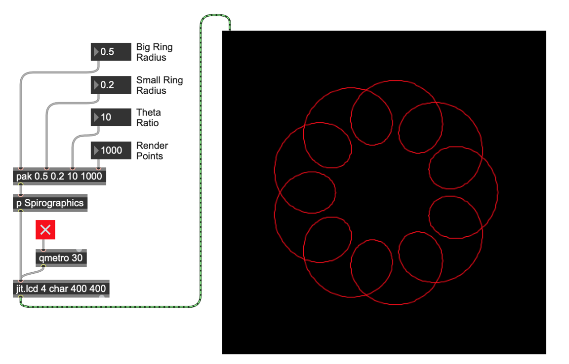
The basics of this patch are pretty straight-ahead: a set of four parameters are needed to control the drawing:
Two radii that set the relative size of the two rings used to create the drawing
A value (theta) that sets a ratio between the two rings
A number that specifies the number of points to plot when we render our results
So, how does our Spirograph work? Simply put, the Spirograph consists of the interaction between two circles. In the real world of a Spirograph set, there’s a large toothed wheel, and a smaller one that can roll around the inside of the larger one (a hypotrochoid) or the outside (epitrochoid) of the larger wheel.
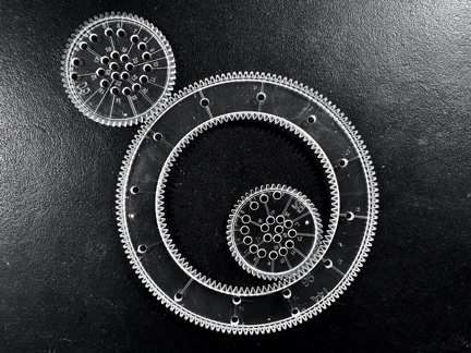
The drawing magic derives from the fact that the gears have differing numbers of teeth, so they spin at different rates. In addition, the smaller wheel contains holes for your pen, which are spaced at equal intervals outward from the center of the smaller wheel, which gives you curves of varying intensity.
We need to start creating our Spirograph patch by getting a handle on the mathematics for calculating the curves, and then translate that understanding into creating some Javascript code to do that for us. A little quality googling time really paid off - there is a beautifully explained online article on creating Spirograph drawings using Javascript by by Chris Maissan. Reading through it wasn’t only inspiring – it gave me a clear starting point for the calculations I needed to perform. Here are the basics (and I’d like to thank Chris for his permission to use the snapshots from his interactive web page).
To draw the inner circle, you can use this formula to plot x and y values within a range of 0. To 2π. The values of cx and cy are the center point of the circle
x = cx + radius × cos(θ)
y = cy + radius × sin(θ)
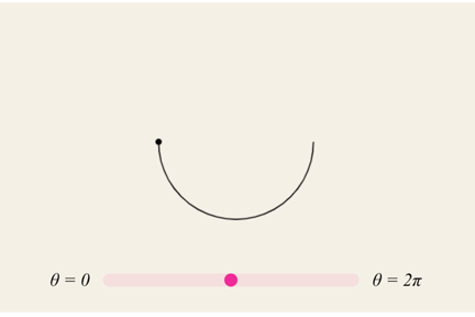
The outer circle should have its center on the outer edge of the inner circle. To do that, we use the value of the initial calculation as the center point for the outer circle
x = cx + radius1 × cos(θ) + radius2 × cos(θ)
y = cy + radius1 × sin(θ) + radius2 × cos(θ)
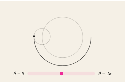
The next calculation is where the magic happens – to simulate the different number of teeth in the inner and outer wheels of the Spirograph, we replace the theta value for the second circle by a ratio. The result is that the ratio determines the number of “spins” of the gear of the Spirograph.
x = cx + radius1 × cos(θ) + radius2 × cos(θ × ratio)
y = cy + radius1 × sin(θ) + radius2 × cos(θ × ratio)
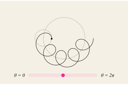
I’d strongly encourage you to visit Chris' website to see the interactive versions of these images and watch them in action for yourself. They were an invaluable starting point for realizing these patches.
Armed with this knowledge, it's time to fire up the Max js object and try to implement this in Max.
Formulas to Code
We're going to create some Javascript code that takes the four parameters from the parent patch and calculates the points to plot as our virtual inner/outer wheel "turns."
To do that, we'll need to do some basic Javascript housekeeping: We set our code to automatically update when it’s saved, and create an object with a single inlet and a single outlet.
Following that, we need to create a constant for use in our calculations, and declare the global variables we’ll be working with.
In the visualization examples we were looking at on Chris Maissan's website, everything was calculated in the range 0. – 2∏ (6.28318), so we'll need to work with that value. Javascript’s math library only includes Math.Pi as a constant, but that’s not problem. We can calculate the value by multiply the Javascript constant Math.PI by two and declare it as a constant.
// Max js object setup
autowatch = 1;
inlets = 1;
outlets = 1;

// constants
var TWOPI = 2 * Math.PI;
Next, we’ll set default values for the size of the radius of the large (outer) and small (inner) circles/wheels for our spirograph. As you'll see, calling them "large" and "small" isn't exactly right, since - as we'll see later on - or "large" parameter value can be smaller than the "small" parameter value and produce interesting results.
In addition, we’ll add a default value (smallRatio) we’ll use for a number of the functions we’ll use to set our plotting values.
The renderpoints variable represents the number of points we’re going to draw to graph our spirograph. In the data visualizations we saw above, the calculations were done at a high resolution. For our patch, we’re going to choose the number of points we’ll use to plot the spirograph. While we obviously would normally use a high number for the number of rendering points, there are some interesting things we can do by experimenting with different resolutions, too.
Knowing the number of render points also allows us to set the amount by which we increment/offset each point calculation as we make our way from 0 to 2π. We calculate that amount (the variable renderstep) by dividing the range (2∏) by the number of points we want to render, and we’ll add use that amount as an increment in the for() loop that does our calculation of each point to render.
Here's a listing of the global values we're going to be working with (along with the defaults we set for them):
// global variables
var largeRad = .70;
var smallRad = .15;
var smallRatio = 10;
var renderpts = 1000;
var renderstep = TWOPI / renderpts;
The body of the program itself is a function – bang() – that takes the current settings for our global variables and outputs a set of x/y vector locations in the range of -1.0 to 1.0. The number of vector locations in the output is set by the renderpts variable.
Inside the bang() function, we’ve got several sets of variables used for the function’s calculations
A pair of variables that represented the last calculated x/y output position
The variables used for the drawing calculations (tmp and the theta value that sets the number of “gears in the wheel”
The starting points for the calculation (stx, sty), calculated based on the size of the small and large radii
A flag set when the calculations are started
// the bang function renders the current settings into a set
// of vector locations in the ranges of -1.0 thru 1.0
function bang() {
    var x, y;            // calculated dimensions
    var tmp, theta;            // variables for drawing calcs
    var stx, sty;            // variables containing the starting points
    var started = 0;        // 'first time' flag
To calculate the coordinate values we need to plot our output, we're going to use a for() loop. Using the computed renderstep value as an increment, the loop starts by outputting the message 0, point, followed by the calculated x/y coordinates. Calculating those x/y coordinates will look familiar to you if you’ve looked at Chris Maissan’s web page equations. Here’s the version from his website again:
x = cx + radius1 × cos(θ) + radius2 × cos(θ × ratio)
y = cy + radius1 × sin(θ) + radius2 × cos(θ × ratio)
And here’s the for() loop code from the js object that does the calculation
for (theta=0; theta<TWOPI; theta+=renderstep) {
        // calculate the drawing position
        tmp = theta * smallRatio;
        x = largeRad * Math.cos(theta) + smallRad * Math.cos(tmp);
            y = largeRad * Math.sin(theta) + smallRad * Math.sin(tmp);

            if (started) {
            // send out the current point
            outlet(0, 'point', x, y);
        } else {
            started = 1;

            // send out the start message along with the
            // first drawing location (the start point)
            outlet(0, 'start', x, y);

             // store the start point for later
            stx = x;
            sty = y;
        }
    }

     // send out the end message along with the
    // original start point (to complete the drawing)
    outlet(0, 'end', stx, sty);
}
Whenever the bang() function is triggered (i.e whenever one of the four input parameters from the parent patch is changed), a starting message is sent out of "outlet 0" (the first/only outlet) from the js object as a message in the form:
start <first-stxvalue> <first-sty-value>
That calculated pair of coordinate values is stored as the stx and sty variables for use at the end of drawing. Then, as the for() loop runs, the result of each of the calculations is sent out the js object as a message in the form:
point <x-coordinate> <y-coordinate>
When the incremented renderstep value exceeds 2∏, a final message in the form:
end <last-stxvalue> <last-sty-value>
is output, using the stored positions, to complete the drawing and return us to the starting point.
The rest of the Javascript code contains a number of small functions used to set the radius of the “small” and “large” rings and constrain those input values to a reasonable size, a simple function that sets and constrains the actual ratio of the small ring rotations per large ring rotation, and the function that calculates the number of steps/points to render (calculated by dividing the number of points by 2∏ (6.28318). Here's an example of one of those functions:
// set the radius of the 'large' ring
function setLargeRadius(v) {
    if ((v > 0.01) && (v < 0.99)) {
        largeRad = v;
    }
}
Doing a Little Drawing
Now that we've got our Javascript code set up, let's walk through the Spirograph_lcd.maxpat patch.
Each of the four variables our patch uses are sent to a pak object, which will output a four-item list whenever any of the input variables changes. The resulting list is sent to the p Spirographics subpatcher. Here's the inside of the subpatcher:
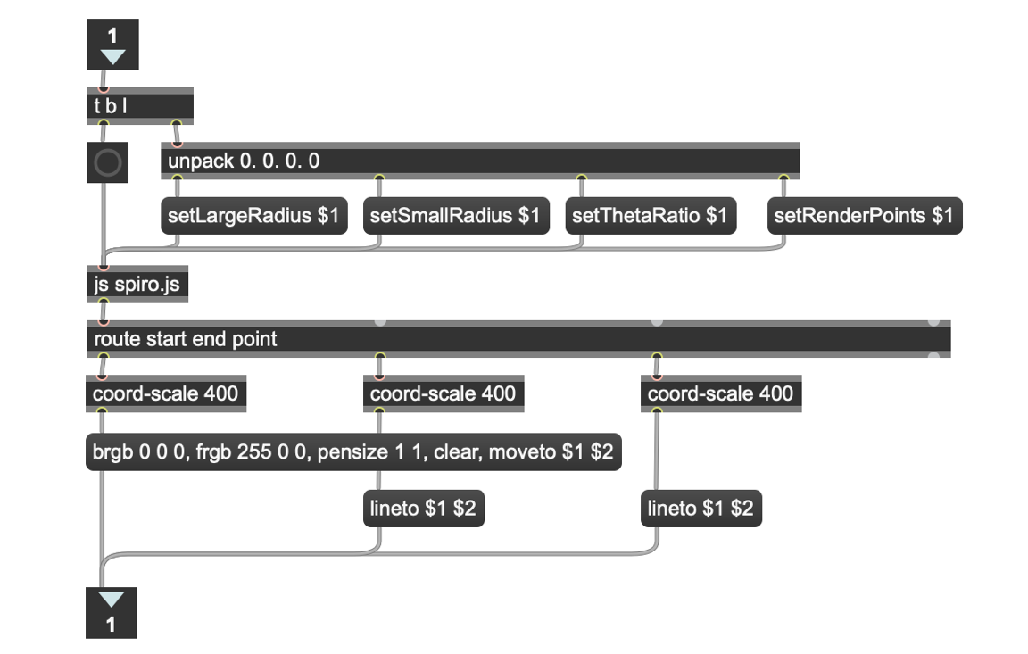
The trigger object takes the four-item list from the parent patch and unpacks the list, setting each of the variables (LargeRadius, SmallRadius, ThetaRatio and RenderPoints) used in our Javascript code. After that's all unpacked, the trigger object sends a bang message to the js spiro.js object, which does all of our calculations for us.
The js spiro.js object outputs one of three slightly different messages that we use in plotting our results:
A start message, whose co-ordinates are always the same (start
A point message for each of the rendering steps which contains the x and y coordinates of the point to plot
An end message whose co-ordinate are also always the same (start, etc.)
The messages for each point to plot from the js object are sent out the route object’s point output, where the list output constructs a lineto message that draws a line between the previous point and the new one. However, there’s one bit of housekeeping we’ll need to attend to for a good plot to the jit.lcd object: The output of our Javascript code produces x and y coordinates in the range of -1.0 to 1.0. Since that will produce a really tiny output image for a jit.lcd object, we’ll need to scale our output lists to plot the output over a more easily visible range. The coord-scale abstraction handles us for that using a vexpr object to process the list input to provide output in a more visible range (400 points, in this case).

The messages for each point to plot from the js object are sent out the route object’s point output, where the list output constructs a lineto message that draws a line between the previous point and the new one.
However, there’s one bit of housekeeping we’ll need to attend to for a good plot to the jit.lcd object: The output of our Javascript code produces x and y co-ordinates in the range of -1.0 to 1.0. Since that will produce a really tiny output image for a jit.lcd object, we’ll need to scale our output lists to plot the output over a more easily visible range. The coord-scale abstraction handles us for that using a vexpr object to process the list input to provide output in a more visible range (400 points, in this case).We use the first of those now-scaled output messages (the start message) to set up our jit.lcd object to begin drawing. When a start message is received, we output the message brgb 0 0 0, frgb 255 0 0, pensize 1 1, clear, moveto $1 $2 to do the following:
We set the background and foreground colors for our display using brgb and frgb messages respectively
We set the size of the line drawn in the display using the pensize message
We clear the current display
We set the point to begin plotting our output with the moveto $1 $2 messageThe end of the js object’s calculation sequence draws a line segment to the point where the original calculation started to complete the drawing
The output of the p Spirographics subpatcher is then sent to the jit.lcd external we use to do our drawing and display. Here's how the sequence of start, point, and end drawing commands to the jit.lcd object work: We use the first of those now-scaled output messages (the start message) to set up our jit.lcd object to begin drawing. When a start message is received, we output a series of messages (separated by commas in the message box) the message brgb 0 0 0, frgb 255 0 0, pensize 1 1, clear, moveto $1 $2 to do the following:
The messages brgb 0 0 0 and frgb 255 0 0 set the background and foreground colors for our display.
The message pensize 1 1 sets the size of the line drawn from point to point in the display.
The message clear clears the current display
The message moveto $1 $2 draws a line to the current coordinate point.
After that, the messages for each further point to plot in the form moveto $1 $2 draws a line to the next coordinate point.
The end of the js object’s calculation sequence draws a line segment to the point where the original calculation started to complete the drawing.
Using the Spirograph
We've now got a working Spirograph. It's time to experiment with the parameters available to us! You'll be surprised at the range of possible outputs. Here are a few interesting things to consider:
Your ability to set different theta values lets you control the number of "loops" in the spirograph output. To specify a particular number of loops, just add 1 to the number of loops you want, and set the theta to that number:
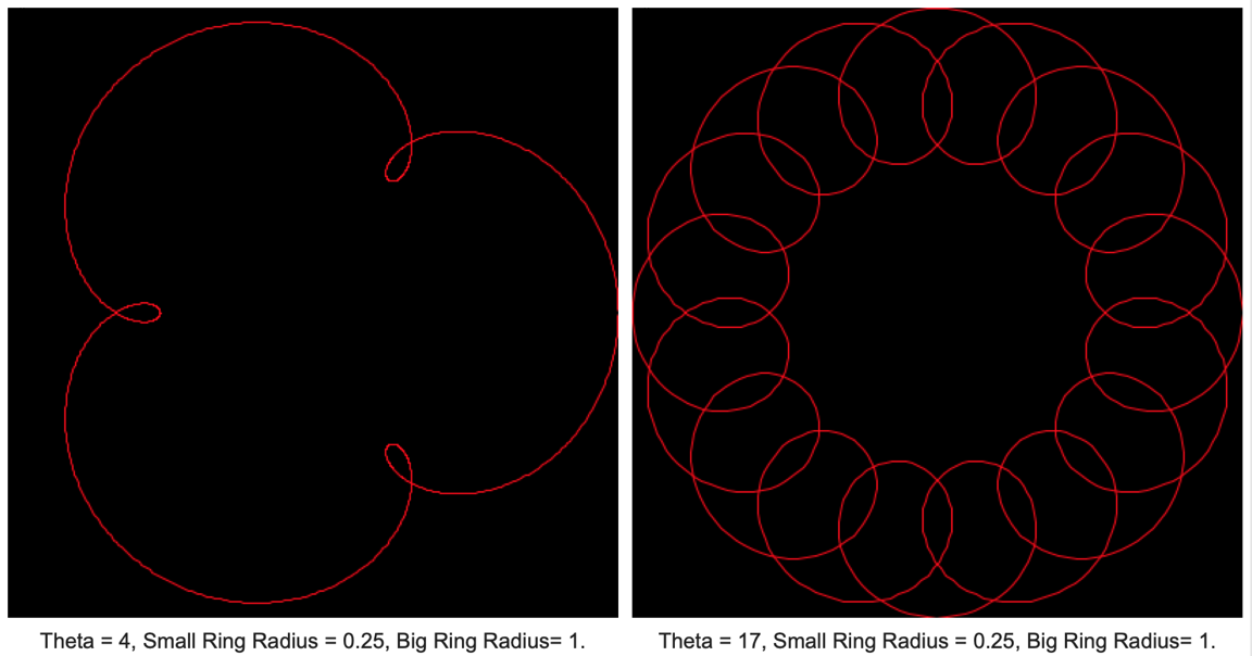
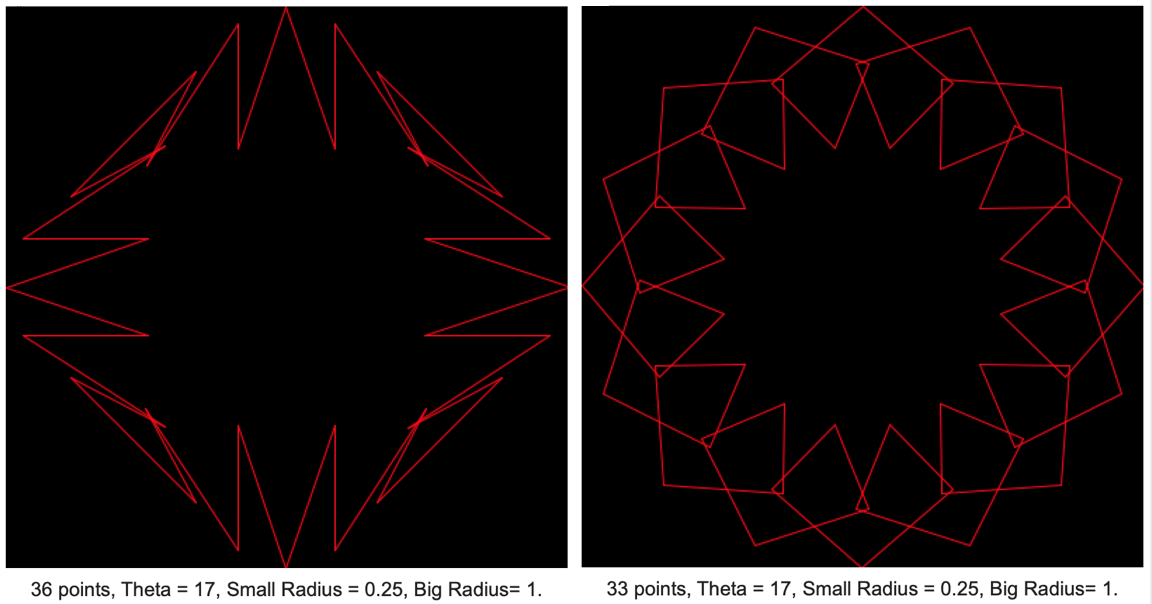
You can experiment with setting the number of render points for your calculations (Remember: the calculation will be executed in the low-priority queue, to setting a very high number of render points will slow down your output). You might want to experiment with the relationship between the theta values and a lower number of plotting points.
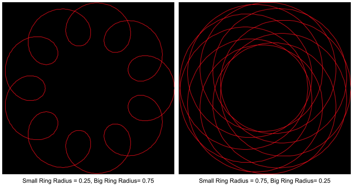
While we've used the terms "Small Ring Radius" and "Big Ring Radius," they're actually independent values - explore reversing the parameter values, or using the same value for both radii:
You could also modify your patch to set up two separate drawing passes (i.e. two js spiro.js sets of calculations) drawn to the same jit.lcd object with different color pens....
You get the idea. Have some fun! Next time out, we're going to investigate implementing a Spirograph using OpenGL, and add a third dimension to our visuals. See you then!
by Darwin Grosse on December 1, 2021

